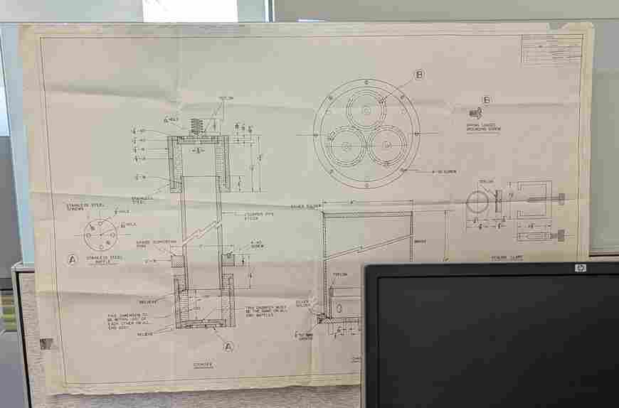
The purpose of this program is to allow accurate measurements of distances and angles in photographs of physical objects with planar features. For instance, the width and height of windows in a building, the relative lengths of ships out at sea, and sizes of objects set on a desk. In a sense this is a continuation of the theory presented in the Image Straightener article, because back then despite a functional result I did not reach a satisfactory resolution to the underlying question: is it possible to determine the projection of a square (equal sides) from solely the outline of a rectangle in a plane that has been photographed? In the Image Straightener I included an aspect ratio adjustment slider, which could be used to define the shape of a square after defining the plane, but is it possible to not require such an adjustment? This is at least true for a photograph of a plane taken with the camera sensor parallel to the plane, such as a scanned sheet of paper, because then a square has equal side lengths in terms of pixels. Can this be extended to planes that are tilted and rotated with respect to the camera? It turns out that this is possible, forming the basis of the algorithm used in the Photogrammetry program.
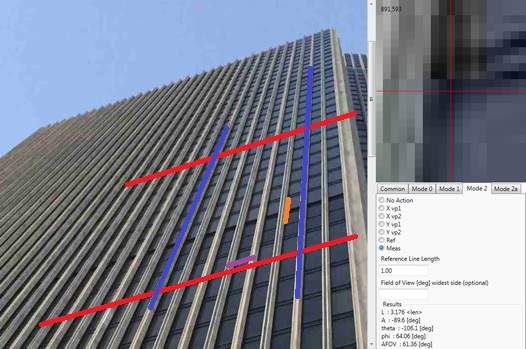
A screenshot of the program used to measure an object plane defined by the facade of a tall building. Lines are drawn thicker for clarity.
Tools and actions are selected in the lower right corner, by first clicking a tab, then a button in the tab. With a tool active, it is possible to click on the image to place a line endpoint. A left mouse button click places the first endpoint, and a right mouse button click places the second endpoint. In the upper right corner, a magnified view of the image appears to allow positioning of the selection to within a pixel. After an endpoint has been placed with the mouse, it is possible to use the arrow keys to adjust the endpoint, and the spacebar causes the selection to switch to the opposite endpoint, so that fine adjustment of a line can be achieved with the keyboard.
Begin by loading or pasting an image, using the corresponding button in the Common tab. Note that pasting an image may not work reliably, due to a bug in the .NET framework. After the image is visible, click a tab for the desired measurement mode. Then click one of the radio buttons in the tab to place a line in the image, and place the line using the left and right mouse buttons. (To simplify the interface, image axes are referred to as X and Y, whereas they correspond to i,j in the Theory section below.) The lines should be placed in the order of the radio buttons, from top to bottom. Each line will need to be placed for the calculation to proceed. Once all the lines are placed, the calculation result will show up at the bottom of the tab. Numeric values required for the calculation may be entered in the text boxes. Already-placed lines may be edited by clicking the associated radio button and then somewhere in the image.
The presentation here was aided by these useful sources: Handprint: Two Point Perspective, Mathematics of Perspective Drawing, and a stackexchange discussion on Properties of Measuring Points in perspective drawing.
A photographic camera can be idealized as a device projecting points from the physical object through an aperture onto an image sensor plane. The object plane will refer to a plane on the physical object, while the image plane will refer to the pixels of a photograph of said object. A square tile will always be square in the object plane, but may look like a more general quadrilateral in the image plane depending on the angle from which the photograph is taken. In 3D space with orthogonal X,Y,Z axes, define the image plane as parallel to the XY plane and passing through Z=Di. The aperture will be located at the origin (0,0,0). The object plane will be defined elsewhere in the space, and the image of this plane will be projected by drawing lines from each point on the object plane, through (0,0,0), and to a point on the image plane.
Note that this is a planar projection, which is accurate for most photographic cameras, however it is not the only option - for example in a strict planar projection reaching a field of view of 180 degrees requires an infinitely large sensor. Our eyes can see close to this field of view while remaining small because their sensor is curved rather than planar, and various fish-eye lens and full-sphere ("360 degree", or better 4*pi steradian solid angle) camera lenses maintain a flat sensor but use lenses which do not behave as a point aperture. This is also why in paintings a slight deviation from planar projection may look more visually appealing. However a non-planar projection will not necessarily project lines to lines.
It is desirable to minimize the degrees of freedom in the description of this problem, to make the solution more tractable. From considering the above situation geometrically, we can intuit that the rotation of the camera about the Z axis is not important to distance measurements, so we only need to use one rotation angle for the object plane. Define the object plane as passing through (0,0,Dp) and rotated by angle phi about the Y axis relative to the XY plane. If we have coordinates (h,g) in this plane, where h is along the projected X axis in the object plane, and g is along the projected Y axis in the object plane, then we can map to (x,y,z) coordinates by:
[ xp ]   [ 0 ]   [ cos(phi), 0 ]   [ h ]
[ yp ] = [ 0 ] + [     0   , 1 ] * [ g ]
[ zp ]   [ Dp]   [ sin(phi), 0 ]
For the choice of aperture location at (0,0,0), all projection lines will be of the parametric form:
[ x ]   [ a ]
[ y ] = [ b ] * t
[ z ]   [ c ]
For a point on the object plane, the values (a,b,c) will define the projection line, and two values of t will correspond to a point on the object plane and a projected point on the image plane. We know that in the image plane zi=Di, and in the object plane we know zp, so the t value for the projected point on the image plane is t=Di/zp. From this we can determine the image point:
[ xi ]   Di   [ xp ]
[ yi ] = -- * [ yp ]
[ zi ]   zp   [ zp ]
Then within the object plane, we have lines drawn at 90 degrees to each other, defining a rectangular grid, which may be rotated by angle theta about the plane normal relative to the projected X axis. This grid is purely a visual indicator, because the physical distance measured in the object plane is independent of theta (we may rotate the grid as we like, the projection is a function of Di,Dp,phi only). If we define the physical coordinates in the object plane as (i,j) along the axes as rotated by theta, we can relate this to (h,g) of above by a standard 2D rotation matrix:
[ h ]   [ cos(theta), -sin(theta)]   [ i ]
[ g ] = [ sin(theta), cos(theta) ] * [ j ]
Then combining the two rotations and the projection relation above, we can obtain the image point (xi,yi) in terms of object plane axes (i,j) as follows
            (cos(phi)*cos(theta))*i - (cos(phi)*sin(theta))*j
xi = Di * ------------------------------------------------------
          (sin(phi)*cos(theta))*i - (sin(phi)*sin(theta))*j + Dp

                     (sin(theta))*i + (cos(theta))*j
yi = Di * ------------------------------------------------------
          (sin(phi)*cos(theta))*i - (sin(phi)*sin(theta))*j + Dp
Generally there will be another rotation of the image about the Z axis, which is equivalent to rotating the image in-plane, but this complicates things and does not impact the results as we will apply them. Similarly a line at constant i or at constant j with varying theta can describe any line in the object plane or image plane.
Note that by similar triangles in the projected image, changing Di is equivalent to a uniform magnification of the image about (0,0,Di) or setting the scale for (xi,yi), and changing Dp is equivalent to a uniform magnification of the object within its plane about (0,0,Dp) or setting the scale for (i,j). The two magnifications are not identical (at non-zero phi) due to foreshortening. This is supported by the equations: xi and yi are proportional to Di, while multiplying i,j,Dp by the same scalar leads to no change in (xi,yi).
Now define a parametric line in the physical plane:
[ i ]   [ a ]       [ c ]
[ j ] = [ b ] * t + [ d ]
Then we can substitute this in the above equations for (xi,yi)
            ((cos(phi)*cos(theta))*a - (cos(phi)*sin(theta))*b)*t + ((cos(phi)*cos(theta))*c - (cos(phi)*sin(theta))*d)
xi = Di * ----------------------------------------------------------------------------------------------------------------
          ((sin(phi)*cos(theta))*a - (sin(phi)*sin(theta))*b)*t + ((sin(phi)*cos(theta))*c - (sin(phi)*sin(theta))*d) + Dp

                              ((sin(theta))*a + (cos(theta))*b)*t + ((sin(theta))*c + (cos(theta))*d)
yi = Di * ----------------------------------------------------------------------------------------------------------------
          ((sin(phi)*cos(theta))*a - (sin(phi)*sin(theta))*b)*t + ((sin(phi)*cos(theta))*c - (sin(phi)*sin(theta))*d) + Dp
We then solve for the limit (xvp,yvp)=(xi,yi) as t approaches infinity:
           cos(phi)
xvp = Di * --------
           sin(phi)

              1       sin(theta)*a + cos(theta)*b
yvp = Di * -------- * ---------------------------
           sin(phi)   cos(theta)*a - sin(theta)*b
This is an interesting result - note there is no dependence on (c,d) or Dp, and xvp is independent of theta. The "vp" stands for vanishing point - all parallel lines in the object plane will appear to intersect at the vanishing point in the image plane. Further, all vanishing points will exist along a line in the image plane, which we may call the horizon line. In our definition this line is at constant xvp (parallel to the Y axis), but in a photograph it may be rotated about the Z axis as well - in that case we can rotate the photograph about its center to make the horizon line parallel to the Y axis so the definitions here apply. The horizon line is the intersection of the image plane with a plane parallel to the object plane and passing through (0,0,0).
There is another abstract line which is the intersection of the image plane with the object plane, and along this line the physical lengths of the image plane and the object plane are equal. This may be visualized as extending the size of the camera sensor until the intersection is visible in the photograph, and then the pixel pitch of the sensor will match the physical size of the object features. This line will not be in the image unless some very strange camera is used, however it is known to be parallel to the horizon line. Because of proportional scaling, any line in the image plane that is parallel to the intersection line and hence to the horizon line, will match the physical size of the object features with some constant scaling factor. This is important because it gives us a "measuring line", where uniformly measured intervals along its length in the image plane will also be uniformly spaced physically in the object plane.
At this point we can sketch an outline for a measurement process:
An issue is that without a specific process for choosing MP, we are not guaranteed that the projection angle within the object plane is aligned with the points of interest. This may be solved by using two MPs, which are chosen so that the associated lines in the object plane are perpendicular. Then any length in the object plane may be composed as a^2+b^2=c^2, where (a,b) are the lengths measured from the two MPs, and c is the desired length. A further concern is that when the object plane projection lines are at differing angles to the intersection line, the projected lengths are scaled unequally. This is presented visually below.
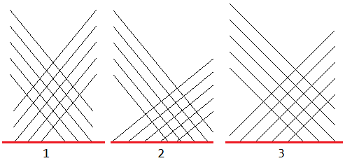
This illustrates the measurement process in the object plane. The choice of two MPs in the image plane determines two angles for parallel lines in the object plane (drawn in black) which are used to project dimensions onto ML (drawn in red). In case 1, the angles are not at 90 degrees to each other, which means projected dimensions are stretched or shrunk. In case 2, the lines are at 90 degrees to each other but they are at different angles to ML, which means i and j dimensions are not scaled equally. In case 3, the lines are at 90 degrees to each other and at equal angles to ML.
The choice of two MPs which project lines at 45 degrees to the ML in the object plane is natural, but how can these MPs be found in the image plane? Using the above formalism, they correspond to the i-axis or j-axis VPs at theta=[45,-45] deg. Call these the diagonal measuring points (DMPs):
            cos(phi)
xdmp = Di * --------
            sin(phi)

             [+-]1
ydmp = Di * --------
            sin(phi)
Now the details of the projection start to matter. Di needs to be related to the pixel pitch of (x,y), which is less confusing if represented as an angular field of view (AFOV) and sensor width of the camera (SW).
Di = (SW/2) / tan(AFOV/2)
The above is represented in physical units but it can be just as well represented in pixel units, where the sensor width is the pixel width of the photograph. Then the xi and yi coordinates are measured in pixels from the center of the photograph. It is interesting that this means the center of the photograph is not an arbitrary point in the planar projection. Rotating a camera to see more of a scene is not equivalent to moving the sensor laterally. The difference is exhibited in tilt-shift lens photography. I had a hard time conceptualizing this, probably because the eye uses a more spherical projection where turning the head is similar to looking at an edge of the visual field, and also because the retina of the eye is always centered with regard to the eye lens, thus we do not have first-hand experience of this phenomenon. To further prove this, I used a camera to take photos of a poster from the same aperture location, but with the camera rotated to place the poster towards the right of the image, center of the image, and left of the image. Then I cropped these three images so that the poster appeared centered in the cropped versions (breaking the assumption that the center of the image is the center of the lens). Try visually estimating the aspect ratio of the poster from these three images: version 1, version 2, version 3. Do you get different results? It may help trying to mentally draw a line that would appear diagonal on the poster. After making a guess for what the actual aspect ratio is, compare it with this in-plane photograph: version 4.
Given AFOV, we have everything we need for Mode 1 operation. With a specified horizon line (HL), we find the shortest distance from HL to the origin to counter possible rotation of the image, and this distance is equal to xdmp. Then from AFOV and the photograph width providing SW, we find Di. From xdmp and Di we solve for phi, and then from Di and phi we solve for ydmp. ydmp is the distance from the point on HL closest to the origin to the two diagonal MPs for the image. Then we use some line parallel to HL as ML, project from the two MPs onto ML, and find a distance as sqrt(d1^2+d2^2). By keeping track of the individual distances (d1,d2) it is possible also to find relative angles between lines in the object plane.
For Mode 2 operation, we have two lines parallel to the i-axis, and two lines parallel to the j-axis, in the image plane. We find the intersections of the two lines in each pair, giving us the vanishing points IVP and JVP. The horizon line (HL) passes through these two points. From here, we may proceed as in Mode 1 when AFOV is provided. However we do not require AFOV because we can make use of the fact that IVP and JVP define perpendicular lines in the object plane. Again per the above, the i-axis and j-axis VPs as a function of theta are given by:
         Di
IVP = -------- * ( cos(phi), tan(theta) )
      sin(phi)

         Di
JVP = -------- * ( cos(phi), tan(theta+pi/2) )
      sin(phi)
Hence from to the origin (center of the image or (0,0,Di)) the lines to IVP and JVP form an angle representing pi/2 or 90 degrees in the object plane. Any other theta, including 45 degrees for (xdmp,ydmp), may be found by using the same tangent scaling. The angle will not be 90 degrees in the image plane because of the foreshortening effect from Di and phi, however we may counter this effect by virtually shifting the origin point of the image along the X axis until the angle from this point to IVP and JVP is 90 degrees in the image plane. This point may be called the view point. Two perpendicular lines through the view point, when intersected with HL, will give two perpendicular MPs in the object plane. Theta may also be determined using the view point. So after finding the view point, we can draw lines through it at +-45 degrees to HL, and obtain the two DMPs without knowing AFOV.
There is another approach that should be mentioned, that follows the measuring points as used in perspective drawing (described in the handprint guide (in turn referencing Brook Taylor's New Principles of Linear Perspective (1719))). If we limit the measured object to being along the i,j axes, we can use specific projecting lines that are not at 90 degrees to each other. Any angle will project a proportional length, but specific angles will have proportionality of unity.
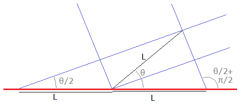
A length L along a particular line (black) in the object plane may be mapped to the same length along the measuring line (red) by projecting along two angles (blue lines), which gives two MPs in the image plane.
There are thus two MPs for each of the i,j axes, which will project a length along those axes to ML. These MPs are defined below. To get a sense for how this looks in an image, I wrote MATLAB scripts to calculate the projection of points in the object plane based on the above variables (projection.m), and to calculate the various VPs and MPs (projection_pts.m).
          Di
IMP1 = -------- * ( cos(phi), tan(theta/2+pi*3/4) )
       sin(phi)

          Di
IMP2 = -------- * ( cos(phi), tan(theta/2+pi*1/4) )
       sin(phi)

          Di
JMP1 = -------- * ( cos(phi), tan(theta/2+pi*1/2) )
       sin(phi)

          Di
JMP2 = -------- * ( cos(phi), tan(theta/2) )
       sin(phi)
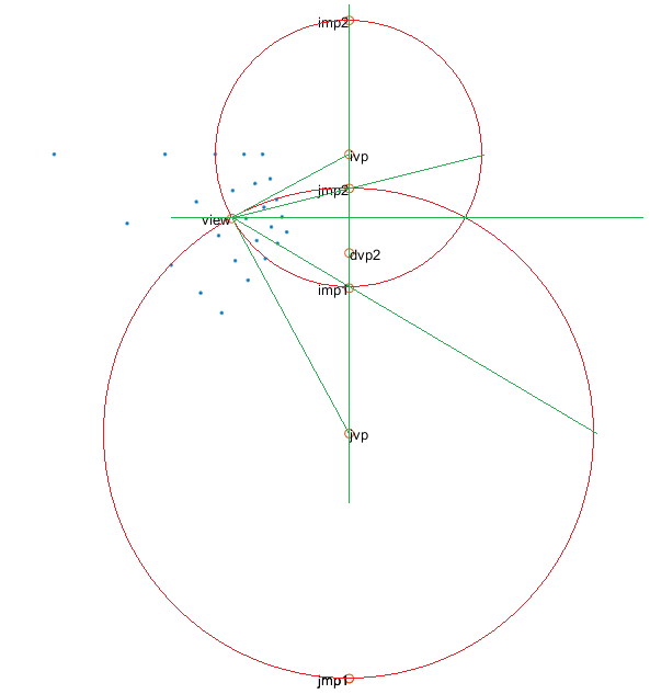
A geometrical construction of the above measuring points. The image shows blue points which are the corners of projected uniformly sized squares (using the MATLAB script above), the two vanishing points for i and j axes, the green horizon line connecting these VPs, the view point where the angle to the VPs is 90 degrees, and the measuring points which have angle offset from theta/2 as described above. Note that in the image plane, the MPs of each axis are uniformly spaced about its VP, illustrated by the red circles, and the circles are centered on each VP and pass through the view point. One of the diagonal VPs is also shown for reference. To get a better visual understanding of the labeled points, try holding a ruler up to the screen such that it traces a line through one of the points and note how the line relates to the blue projected points.
For a general point in the image, it may be projected onto the i,j axes by drawing a line from the opposite VP, and then to find the distance between two points they would both be projected onto both axes, then each axis would have a choice of MP to project that component onto ML. Combining the lengths in quadrature gives the physical distance and angle. For Mode 2a, this approach is used, except the choice of MPs is kept arbitrary because the reference lengths along each axis are given so the scaling does not need to be calculated separately.
Because the VPs of an offset plane will be unchanged, it is possible to use Mode 2 or 2a for offset planes as well, as long as the length reference also lies in the offset plane. If this is not the case, it is possible to measure a length of some transfer object in a perpendicular plane using an in-plane reference, then use that length as the reference in a redefined offset plane. I tried to implement this functionality in a user-friendly manner as another measurement mode, but that ended up requiring more effort than I could justify because the use case seems quite limited. The beginning of this "Mode 3" tab is included in the code files below as Cube2ProjControl.
The approach presented above works mathematically, but it still does not give a clear intuition for what is happening. Even in the code, there are too many separate cases, especially when the intersection points of the vanishing lines are far away, so there should be a more elegant way to approach the problem. This may be done by adding a spherical projection - consider placing a sphere, centered on (0,0,0), and project from the object plane onto this sphere as well as the image plane. (The sphere diameter doesn't matter, because only the relative angles defined by Di,Dp will be pertinent.) Then, what appears as a horizon line in the image plane, makes a horizon circle on the sphere.

A schematic drawing of spherical projection along with the object and image planes. The two planes are shown parallel to each other (phi=0 deg), and the horizon lines would be infinitely far in both planes, but would form a circle on the central sphere, illustrated in green. This horizon circle is parallel to the object plane.
This circle has the same radius as the sphere, meaning that its center is also at the origin, and it may be fully defined by two distinct (and non-opposing) points on the sphere surface. More sensibly, with the horizon circle, we never have to deal with points at infinity. The horizon circle is parallel to the object plane, so if we find a way to obtain the horizon circle from the image plane, we can complete the inverse transformation and measure distances in the object plane. The value of Di for the image plane makes a difference in how we determine the horizon circle, namely how pixel coordinates correspond to angles on the sphere. This is why the angular field of view is a required parameter in Modes 1 and 2. Note that with angular field of view known, there is no longer a requirement for the axes to be perpendicular in the object plane, as any two vanishing points will define a horizon circle. However, if we know that two vanishing points define perpendicular axes, then we have the constraint that on the horizon circle, the two projected vanishing points will form a 90 degree angle through the center of the circle. By this means, we can estimate the angular field of view from the image. This is what the algorithm for Mode 2 does, though staying within the image plane rather than making a spherical projection.
The program executable may be downloaded here (110 KB, requires .NET framework 4.8). C# code files may be downloaded here. Each of the measurement mode tabs is a derived class from ProjControlBase (which extends a Control object), avoiding redefinition of common tasks like adding and adjusting lines.
By using photographs of objects of known size, I have verified that the algorithm works and the results are generally accurate within 0.1 x. Accuracy of 0.01 x can be reached, but requires "pixel-perfect" adjustments of all the reference lines. I find that typically an inaccurate result is due to slight misplacement of the lines defining the axis VPs (IVP and JVP in the Theory section). The AFOV calculation gives values within 5 degrees of the true value with well positioned planes (where phi and theta are both near 45 degrees), and I have found that adjusting the VP lines in Mode 2 until the calculated AFOV matches the true value will lead to more accurate measurements (versus entering the true value as an input, because then the algorithm is less sensitive to small deviations but the lines are still mathematically mismatched). When VPs are far away and their reference lines nearly parallel, and when measurements are done close to the horizon line, accuracy decreases as expected. I tried to add an accuracy warning when the result is deemed sensitive to small changes, but there proved to be too many odd cases where the warning was not working as expected, so this feature was removed (except for one in Mode 2a), and accuracy judgements are left to the user. Overall, I would call this project a success. I use this program on a fairly regular basis, though mostly in Mode 0, to read out unlabeled dimensions from scans and drawings.